In my last [post] I talked about Optical Character Recognition and how I managed to get a solution working using machine learning, particularly using the nearest neighbour algorithm. In this post I will briefly explain how the NN algorithm works and then introduce another two pattern recognition algorithms which I used to solve the OCR problem and compare their strengths and weaknesses.
Live demo can be accessed [here].
In a future article, I will implement the same algorithms using ML.NET and see if I get better results than my own implementations. So stay tuned!
1. Nearest Neighbour
The algorithm is based on a distance metric such as the Euclidean Distance which is used to find the closest similarity (nearest distance) among a set of vectors. Let’s assume in this case we have an array of integers and we want to compare this with other arrays of integers to determine which one is the most similar to our own array of integers. A loop would go through each of the arrays one by one and make a comparison using the following simple formula below to obtain the euclidean distance.

At each iteration, every integer from array 1 is represented as x and every integer from array 2 is represented as y. In C# code, the following formula would translate to something like [this]. By applying this formula to compare the array of integers against all the other arrays inside the data set, the array which produces the shortest distance as result is considered to be the most similar to our array and this is how it was possible to solve the OCR problem in my previous [post], hence by comparing the array of bits produced by the scribbling on a canvas against all the other OCR images inside the CSV files.
2. K-Nearest Neighbour (k-NN)
In combination with nearest neighbour, a very powerful solution which can be used to optimise the accuracy of the nearest neighbour is the k-NN algorithm; a non-parametric supervised learning method used for both classification and regression predictive problems.
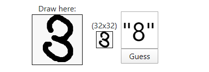
The k-NN rather than classifying the nearest neighbour by shortest distance metric, it takes the closest K neighbours and forms a majority vote among them to determine which character occurs the most times (K being any number). So basically going back to the OCR problem, let’s imagine that “3” is the number we are trying to predict by using the Nearest Neighbour and we get Euclidean Distance of 0.2 on a character which is a “3” and 0.19 on a character that is an “8”. This can very much happen if the character is not written very clearly and thus it gets mistaken for a number with similar pattern attributes.

What the k-NN does basically, rather than choosing the result with shortest distance; it takes the top four or five (K) with shortest distance which are found. This way a vote can then be made and determine the likelihood from the majority. For the sake of our example, we could get the following for K=4:
{ 1.9 = “8”, 0.2 = “3”, 0.21 = “3”, 0.24 = “3” }
This means that although the result with shortest euclidean distance relative to our number is an 8, there are another 3 results which indicate it’s a 3 and therefore the majority vote concludes that it is in fact a 3. This improves slightly the predictive performance over the classical nearest neighbour. A C# implementation of the k-NN can be found [here].
3. Multi-Layered Perceptron
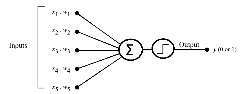
The Multi-Layered Perceptron originates from a single perceptron node which takes a set of input values as parameters and then produces a binary output (usually 0 or 1). At each input node, a randomly generated weight value (ex: -0.5 to +0.5) is set and multiplied to the input value. The totals are then summed together in a connecting node and finally the total is produced using the sigmoid function a.k.a the step function (or activation function).

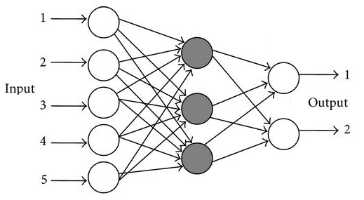
Of course the perceptron approach works very well when dealing with linear separation for example when determining whether an object is a car or a truck (separating only 2 types), but in our case the OCR problem is more complex than that. For this reason, multiple perceptrons can be combined together to form a neural network which will be able to identify 10 different characters, hence produce 10 different output types.

This approach could work even if multiple middle layers (called hidden layers) could be connected in between each with their own weight value and values summed together from back to front (feed forward). However the a neural network is usually implemented with a back propagation function which goes backwards and corrects the values at each iteration during training phase in order to minimise the resulting error for that particular value and thus drastically improving the performance on the prediction results. Back propagation is quite complex to understand but many tutorials are available online which go in depth with the explanation.
For our OCR solution, a MLP algorithm classifier example in C# has been implemented and can be found [here]. The following configurations have been applied.
- Input Layers (64): The OCR data is represented in a 64 bit binarised numeric value.
- Output Layers (10): The possible classification of digits 0 – 9.
- Hidden Layers (3): By trial and error it turns out 3 layers give the most accurate results.
- Hidden Neurons (52): “The number of hidden neurons should be 2/3 of the input layer size, plus the size of the output layer”, Foram S.Panchal et al (2014).
- Momentum (0.4): The coefficient value multiplied by the learning step which adds speed to the training of any multi-layer perceptron.
- Learning Step (0.04): The constant used by algorithm for learning, 0.4 gave the best results while fine tuning although for smaller datasets 0.06 also worked very well.
- Least Mean Square Error (0.01): The minimum error difference to get in training precision before stopping.
- Epoch (500): The number of times to repeat the back-propagation during training to get the weights adjusted correctly. The higher the value the more precise the character recognition but the slower the performance. NB: Setting this value higher than 500 seems to make insignificant difference in the output accuracy for the data set which we are working with.
- Function: Sigmoid function has been used as most practically used worldwide.
When passing the two-fold data through the perceptron, the training method might take a bit long to complete since it will need to iterate too many N times for each character given. For this reason filtering has been applied to limit the number of training data for each represented digit from 0 – 9 but is has been observed that the smaller the data set for training passed although it shortens the processing time, it reduces the percentage accuracy of the result.
Results Comparison
Below are the accuracy performance results based on a 2-fold test. But perhaps the accuracy can be tested manually on the live demo page [here]. Which one gets it right most of the time for your handwriting?
| Algorithm | Performance | % Accuracy |
| KNN | 2760 / 2810 | 98.22% |
| NN | 2755 / 2810 | 98.04% |
| MLP | 2727 / 2810 | 97.04% |
Conclusion
The nearest neighbour and k-NN functions have shown by far the highest accuracy achievement in the smallest amount of running time however such algorithms, being non-parametric kind; lack the ability to learn and therefore their processing requires a training dataset to be available at all time. On the other hand, the multilayer perceptron is able to learn and produce a neural network with adjusted weights over a span of time which then uses to classify characters without the need to the original training set.
Although such method takes a very long time to run compared to the other methods, the weight adjustment values can be saved in a file after the training has been completed and then use only the saved adjusted weights from the file to run the OCR classification almost instantly. Theoretically, the MLP method has also the potential that more accuracy can be achieved when fed a larger training dataset and finer tuning of the other parameters such as epoch and learning step.
References
1. Multi-layer Perceptron Tutorial
http://blog.refu.co/?p=931
2. Multi-Layer Neural Networks with Sigmoid Function
https://towardsdatascience.com/multi-layer-neural-networks-with-sigmoid-function-deep-learning-for-rookies-2-bf464f09eb7f/
3. Review on Methods of Selecting Number of Hidden Nodes in Artificial Neural Network
http://www.ijcsmc.com/docs/papers/November2014/V3I11201499a19.pdf