Author: dgrixti

Transitioning Forking to Queuing using RabbitMQ

Post author By dgrixti
Post date 31 March 2022
No Comments on Transitioning Forking to Queuing using RabbitMQ

A while back, at my current position I was assigned to investigate what seemed a really complex problem at first but slowly as I gathered more information I managed to put in place a number of steps to resolve it. Here I will detail the process which I took in order to go from being completely oblivious about a serious performance problem in production to ultimately resolve it and making the system more scalable along the way.

Some technologies covered in this post are RabbitMQ and PHP 7.4.

Problem Report

In a nutshell, the company I work for hosts these online video slot games tournaments in which thousands of players participate and play against each other with a leader-board scoring system. The incidents team from their initial analysis, have reported that from time to time, whenever one of those big tournaments finishes, the CPU on the production server spikes to 100% and the server eventually comes down. The IT have reported that this seems related to a staggering spike in PID processes which suddenly appears on the Linux server and never seem to go down consuming all the resources of the machine.

Problem Analysis

After taking a first look at the code, it was clear that the ending of these tournaments is handled via a cron-job which is executing every minute or so and then for each player participating in a tournament, a series of events are run to calculate the leader-board structure and the prize payout. In our case, we are working with PHP 7.4 and PHP is a single thread language therefore in order to achieve parallel asynchronous tasks, the [popen function] is used to create multiple forks on a separate process (PID). This seemed to be the root of the problem because a few years back when this code was created, one was not accounting for a tremendous growth of users and therefore the code worked well until hundreds of users were participating and thus creating hundreds of PIDs on the server once a tournament finished. Now with thousands of users, the situation is very different.

Possible Solutions

The goal at this point was clear: we need to limit the number of PIDs which get executed on the server so that thousands of threads trying to access the database at the same time are avoided. A few possible solutions were discussed but in the end, the one which seemed most viable was to start using queues instead of PHP forks. This would take longer to develop and get to production but in the long run it will be the more efficient and most scalable solution.

[RabbitMQ] is the choice of messaging broker at this point because it had already been used for other projects and therefore it was a familiar technology within the company despite a few caveats to be known when using PHP, one example is the [keep connection alive] issue which needed to be dealt with. The [AmqpLib] library for PHP would be used to create the publishers and the consumers.

The Plan

So the plan was to start moving the code which is executing in a forked process into RabbitMQ consumer processes. Using [supervisor] we were able to create multiple consumers of the same process enough to handle the volume of work within seconds but never enough to choke up all the server or database resources.

From the FPM side (web part) or the cron-job side, rather than running the fopen() function, a message was published to RabbitMQ and let the consumers take care of the work thus maintaining the asynchronous architecture.

Before:

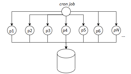
After:

The Result Outcome

Well.. the good news is that after deploying this new architecture, the server stopped crashing and IT were very happy with us, however new problems started to emerge since the original code was not designed to work with a queuing technology. Over the following weeks (and months) we needed to do some further adjustments until all problems went away.

Below are some of the most notable improvements which were laid out to make the system more efficient.

1. Publisher Connections limit
In the error log file, hundreds of the following errors were noticed:

PHP Fatal error:  Uncaught exception 'PhpAmqpLib\Exception\AMQPTimeoutException' with message 'The connection timed out after 3 sec while awaiting incoming data'

It turns out that whenever a publisher needs to connect to RabbitMQ the process is quite heavy as the server needs to exchange 7 TCP packets for each connection to be established [1]. In our case, we needed to create a new connection for each message to get published and at peak times the RabbitMQ server was unable to allocate resources to accommodate all incoming traffic and thus many resulted in timeout. In order to mitigate this problem, we used [AMQProxy] by CloudAmqp which acts as a proxy between the system and the queue and keeps a pool of open connections to the queue and reuses them accordingly when new connections are requested.

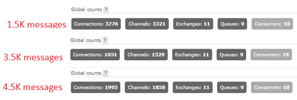
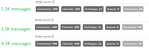
When doing benchmark testing, it seemed at first that the proxy is creating even more connections than necessary, however it was then noticed that the total connections remain stable and do not keep spiking until a deadlock is reached (as was happening before). Below are some illustrations showing the number of connections created on RabbitMQ based on the number of messages published by an internal benchmark tool:

Without Proxy (1 connection per message)::

With Proxy (1 connection per message)::

2. Race conditions
Some code which previously was being forked, was not expected that it could at times take a couple of seconds to finish. As a consequence, we experienced issues with the prize calculations during peak times where some people were not receiving the proper prize amount in the calculation. For the sake of the example, let’s imagine we were doing something like this to calculate prizes:

calculatePrizesPart1();
calculatePrizesPart2();

These are always executed in this order. Then we do

publishToQueue(calculatePrizesPart1());
calculatePrizesPart2();

This would mean that the first part of the code now being published to a queue might finish after the second part. For this reason some parts of the code were revisited to make sure that the entire code blocks are moved to consumers and are executing together or in the right order.

3. Unnecessary SQL bottlenecks
It was noticed that during peak times, the amount of messages arriving to queue was in the hundreds of thousands and it took up to 30 minutes to get emptied. This was causing a lot of problems because clients complain that the prize hasn’t been received in time. After analysing the code, the following logic was noticed:

// Publisher.php
$tournament = getTournamentFromDB($tournId);
$entry = getEntryFromDB($tournament->id, $userId);
publishToQueue('calculate-prize', $tournament->id, $entry-id);


// Consumer.php
processMessage($tournId, $entryId) {
    $tournament = getTournamentFromDB($tournId); 
    $entry = getEntryFromDB($tournament->id, $userId);
    calcPrize($tournament, $entry);
}

Essentially for each prize calculation, we were sending the ID of the objects and then from the consumer run SQL statements again on the database to retrieve the objects again. This caused a heavy load on the database and slowed everything down. To solve this bottleneck, we took the advantage of the RabbitMQ message payload and passed the entire objects inside the message itself and thus eliminating the SQL queries on the consumer side.

// Publisher.php
$tournament = getTournamentFromDB($tournId);
$entry = getEntryFromDB($tournament->id, $userId);
publishToQueue('calculate-prize', $tournament, $entry);


// Consumer.php
processMessage($tournament, $entry) {
    calcPrize($tournament, $entry);
}

Conclusion

The “fork bomb” saga as we call it internally has been quite a pain in the neck for a couple of months for a few people including myself however we have came a long way ultimately resolving it and taking with us a big deal of knowledge on improving a system performance and scalability. I hope this knowledge I’m sharing here can be useful for others too!

References

1. AmqProxy
https://github.com/cloudamqp/amqproxy

2. AmqpLib – The PHP RabbitMQ library
https://github.com/php-amqplib/php-amqplib

Travelling Salesman Problem

Post author By dgrixti
Post date 4 April 2021
No Comments on Travelling Salesman Problem

Part 1

When I was studying AI at the university, I remember this interesting problem called The Travelling Salesman or TSP which we were given to solve in one of the assignments, it was so fun to me that I decided to write this article about it.

Imagine a business man or salesman (or you) wanted to travel to say 4 different cities around the world and come back home, but you wanted to know in which order of travelling from one city to another gives you the shortest route (maybe to save fuel if going by car). In this case, since we’re dealing with 4 cities total, the best way of knowing for sure would be to calculate literally each possible path combination and then measure which one gives the shortest total distance in kilometers.

City #	x coordinate	y coordinate
1.	37	52
2.	49	49
3.	52	64
4.	20	26

The cities are plotted on a graph using the x, y coordinates above.

*The 4 cities we want to travel to plotted on a graph.*

Factorials and Permutations

In order to calculate all the possible variations of the path to travel, we need to get all the cities arranged in all of the possible orders. In mathematics, factorials are used to calculate the total number of possible unique combinations of distinct sequences made from a list of unique objects. The formula for factorial calculation is the following.

Where n is the number of cities in our case, hence it would resolve as follows. The ! symbol followed by he digit indicates the factorial operation.

4! = 4 * 3 * 2 * 1 = 24

This means that we need to figure out 24 different combinations of paths to travel in total, but how do we do this? Well.. we can either do that manually or we can use some math or code instead using what is called a permutation. So by implementing a permutation function in C# in my case, I will be able to get all the 24 possible unique sequences of the cities. The code for this function can be found [here] (which I ripped from an example I found online).

*Creating a path route through all the cities (1, 2, 3, 4).*

When running the permutation for the 4 cities with labels {1, 2, 3, 4}, the result below is produced.

1.	4, 1, 2, 3,
2.	4, 2, 1, 3,
3.	4, 3, 1, 2,
4.	4, 3, 2, 1,
5.	4, 1, 3, 2,
6.	4, 2, 3, 1,
7.	3, 4, 2, 1,
8.	3, 4, 1, 2,

9.	2, 4, 1, 3,
10.	1, 4, 2, 3,
11.	2, 4, 3, 1,
12.	1, 4, 3, 2,
13.	3, 1, 4, 2,
14.	3, 2, 4, 1,
15.	2, 3, 4, 1,
16.	1, 3, 4, 2,

17.	2, 1, 4, 3,
18.	1, 2, 4, 3,
19.	3, 1, 2, 4,
20.	3, 2, 1, 4,
21.	2, 3, 1, 4,
22.	1, 3, 2, 4,
23.	2, 1, 3, 4,
24.	1, 2, 3, 4,

I had some fun with JavaScript illustrating all 24 permutations in an animation. You can have a look [here].

Distance between 2 points

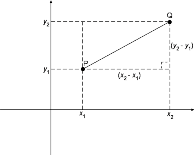
Now that we figured out all the possible unique sequences of the paths we need to solve, we need to find out the total distance of the path. In order to achieve this, the distance from point to point needs to be calculated and then summed. To find the distance between two points (often referred as Euclidean Distance), we need to use the Pythagoras Theorem.

Thus if we define any two points as P and Q, we solve the Euclidean distance as follows.

In C# code this translates to something like the following.

double dist = (double) Math.sqrt(
        Math.pow(city1.x - city2.x, 2) +
        Math.pow(city1.y - city2.y, 2));

The code [here] shows how we calculate the path for each route. Below is the generated results in console.

route: 4, 1, 2, 3, 4, dist: 108.41
route: 4, 2, 1, 3, 4, dist: 118.27
route: 4, 3, 1, 2, 4, dist: 118.27
route: 4, 3, 2, 1, 4, dist: 108.41
route: 4, 1, 3, 2, 4, dist: 102.58
route: 4, 2, 3, 1, 4, dist: 102.58
route: 3, 4, 2, 1, 3, dist: 118.27
route: 3, 4, 1, 2, 3, dist: 108.41
route: 2, 4, 1, 3, 2, dist: 102.58
route: 1, 4, 2, 3, 1, dist: 102.58
route: 2, 4, 3, 1, 2, dist: 118.27
route: 1, 4, 3, 2, 1, dist: 108.41
route: 3, 1, 4, 2, 3, dist: 102.58
route: 3, 2, 4, 1, 3, dist: 102.58
route: 2, 3, 4, 1, 2, dist: 108.41
route: 1, 3, 4, 2, 1, dist: 118.27
route: 2, 1, 4, 3, 2, dist: 108.41
route: 1, 2, 4, 3, 1, dist: 118.27
route: 3, 1, 2, 4, 3, dist: 118.27
route: 3, 2, 1, 4, 3, dist: 108.41
route: 2, 3, 1, 4, 2, dist: 102.58
route: 1, 3, 2, 4, 1, dist: 102.58
route: 2, 1, 3, 4, 2, dist: 118.27
route: 1, 2, 3, 4, 1, dist: 108.41
Winner is: 4, 1, 3, 2, 4, dist: 102.58

It is important to notice that when dealing with such small number of cities, it is common to have routes with the same distance. In fact, although the algorithm says that the winner route is 4, 1, 3, 2, 4 the route with sequence 1, 3, 4, 2, 1 and a few others have the same exact distance of 102.58 km. Nevertheless, this is the shortest route possible of the 24 permutations.

The Factorial Problem

So one might be thinking at this point, OK! problem solved then! brute force can calculate each possible path and we will know which is the shortest path to take. Well… yes, the truth is that if you want to know which route is the absolute shortest, then a brute force algorithm will give the most accurate answer, so why do we need AI? And the answer is the problem with factorials and number of probabilities when dealing with a larger number of cities.

When dealing with even 10 or 20 cities (which isn’t a lot if you think about it) the factorial reaches astronomical values and I’m not even exaggerating. For instance, if we’re dealing with 10 cities:

10! = 1,307,674,368,000

Yes, that is a staggering 1.3 Trillion permutations we need to find and if we had to calculate 1 permutation every 1 millisecond, it would take us over 41 years. What about 20 cities?

20! = 2,432,902,008,176,640,000

That’s 2.4 Quintillion permutations, and would take us over 77 Million years if we calculated 1 permutation every 1 millisecond. Still not convinced? What about 70 cities? Well…

70! = 1.197857167×10¹⁰⁰

Fun fact: scientists have calculated there are between 1×10⁷⁸ to 1×10⁸² atoms in the known, observable universe. This means that if we had write the answer of each permutation that we found on every atom in the universe, we would eventually run out of atoms with about 20% permutations left to find. Anyway! we get the idea…

These are probabilities that not even the world’s best super computers can calculate in a lifetime and therefore Artificial Intelligence can be used to find approximations of the best routes. It’s important to keep in mind that there’s no free lunch in AI and this means it’s probably impossible to ever find the absolute best path when dealing with numerous cities but despite this, some algorithms can help narrowing down the results quite well.

Nearest Neighbour

In another article which I had posted [here] the nearest neighbour algorithm was explained and put to use to find similar patterns by calculating the Euclidean distance between different digit sequences. This can also be applied to attempt resolving the TSP problem by starting at a random city, then calculating which is the nearest city next to that point by shortest distance and move to that one as the next hop in the sequence. This means that the Euclidean distance is calculated from the current city to each of the other cities at each unvisited point at every iteration until all cities are visited.

Using the code [here] I ran the NN algorithm to solve a TSP problem with 51 cities from a [file]. The results I got is the following:

{
distance: 513.610006884723,
city_order: "1, 32, 11, 38, 5, 49, 9, 50, 16, 2, 29, 21, 34, 30, 10, 39, 33, 45, 15, 44, 37, 17, 4, 18, 47, 12, 46, 51, 27, 48, 6, 14, 25, 13, 41, 19, 42, 40, 24, 23, 7, 26, 8, 31, 28, 3, 20, 35, 36, 22, 43, 1, "
}

Who’s to argue with that, right? This is what the algorithm says is the most viable route using the Nearest Neighbour operation, but how can we be sure this is the best? How would the NN compare to the brute force algorithm if we had to run it for the 4 cities in the previous example?

{
distance:108.40979394514636, 
city_order:"1, 2, 3, 4, 1, "
}

Interesting! Although it didn’t pick the longest route, it didn’t pick the shortest either (hence 102.58) so this makes me think it’s not very efficient at finding the most optimal path on the 51 cities either.

Conclusion

In this article the Travelling Salesman Problem is introduced and brute force is used as a first attempt to find the solution. This solution works the best when dealing with a small number of cities but as the number of cities grow, the permutations grow exponentially, so much that no computer would ever be able to solve the problem in less than millions or billions of years.

For this reason, there are some interesting Artificial Intelligence algorithms often known as Heuristics which can approximate and optimise the results in a very short time. The nearest neighbour is one of the simplest of such algorithms which has been explored. In the next part of this article I will be covering other more complex and interesting algorithms of this sort which will help finding a more efficient route to solve the TSP.

Check out the brute force animation I created in JavaScript [here] if you haven’t already.

As always, stay tuned for part 2!

References

1. Pythagoras Theorem diagrams
http://mathsfirst.massey.ac.nz/Algebra/PythagorasTheorem/pythapp.htm

2. Permutations algorithm in C#
https://www.daniweb.com/programming/software-development/threads/349926/c-string-permutation#post1485682

3. N! Factorials
https://en.wikipedia.org/wiki/Factorial

Cloud Hosting

Cloud Hosting – Intro to Docker

Post author By dgrixti
Post date 24 May 2020
2 Comments on Cloud Hosting – Intro to Docker

I am frequently asked by developers who have never put their hands on systems and networking: where does the code go when deploying? how is an application hosted on a server?

In this article I will be creating a dedicated hosting space on a cloud platform onto which I will host a simple ASP.NET demo using Docker. In a future article I will write about hosting your own application from Visual Studio and how to make the application scalable and highly available but for now, I will keep things simple as an introduction.

So stay tuned for my upcoming articles!

1. Creating the server

Whether you have in-house hardware with VMware setup or using a mainstream Cloud Hosting like Google Cloud or Azure, if you want to host your code and prepare it for scaling, the best way to do it is by creating a dedicated server with allocated resources. By this I mean creating a virtual machine somewhere with some ram, CPU and storage, then install an operating system on it and connect it to the internet with a static public IP address. If you manage to do this, congratulations, you’ve basically created a ‘Cloud Hosting’!

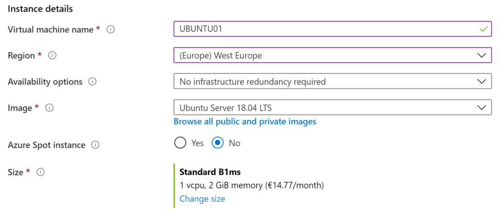
For my example, I will be using Azure for creating a dedicated hosting space, but the process to follow is pretty much the same on any other platform, even if you’re running your own hardware and virtualisation software at work. The first step, is creating a new virtual machine, and in my case; from the Azure dashboard I will create a new Linux virtual machine.

1.1 Resources

In the next step, some resources need to be allocated and of course, the more resources you allocate, the more you pay and therefore the right balance needs to be considered when creating virtual machines. For my project’s requirement I will go with 1 vCPU and 2 GB Ram which for a Linux system this is more than enough. Ubuntu Server is my favourite Linux OS to work with but all other Linux variations are pretty similar if you’re still learning.

1.2. Remote Access

The next step is defining how you’d access this machine remotely from your working or personal computer. When working with Linux Server the best tool for access in my opinion is Putty, with this tool you can create a public/private SSH key pairs using a sister tool called PuttyGen and use these for setting up an SSH access to the virtual machine.

Of course if you’re working on dedicated VM software, you will instead install the Ubuntu Linux manually from an ISO image and then create your authentication as part of the installation process. Nevertheless, Putty can still be used to access the virtual machine with normal username and password in this case. Look up creating public and private keys with Putty and PuttyGen if you’re not familiar with this and then place the public key in Azure and private key in your Putty application.

1.3 Storage

Standard HDD is pretty cheap and works well enough for my exercise but consider SSD storage when planning a system with high IOPS such as database machines.

1.4 Networking

As the for networking configuration, a huge convenience of using online cloud platforms like Google Cloud and Azure is that you get most of the networking configuration done automatically. When working with a dedicated VMware setup however, you will need to make sure to assign a private IP to the machine from your subnet pool and make sure to add the IP to your firewall.

A public IP when will need to be assigned with a NAT rule on the firewall to associate the private IP of your virtual machine with a public IP which is reachable externally from the internet over HTTP. Make sure that inbound HTTP and HTTPS ports are open for this public IP on the firewall and hence port 80 and 443. Also port 22 needs to be open if you want to connect through Putty later on. In this case, on Azure when you hit create you’ll automatically get assigned a private and public IP to the host machine and can be found in the dashboard.

2. Setting up the server

Now that the machine is created and associated to a public IP, we can use Putty to connect through SSH and start setting up the server. If you’re not used to working with strict command line interface, don’t worry, it doesn’t take much to get used to it and trust me, when it comes to Linux it’s way better to learn using the command line rather than the GUI. However if you really want a GUI, you can lookup how to install the GUI on Ubuntu and then use a tool like X2Go to access it remotely.

The first thing to do when accessing a Linux machine the first time is run the update command so that then you can start installing some tools.

$ sudo apt-get update

2.1 Install Docker

At this point, since we’ve created a hosted server and have access to it, we could simply install a web server like NginX or Apache, copy our code on the web server’s directory and run our website through the public IP on port 80 and it would just work fine. Well.. if you had a very simple application with just HTML and CSS it would work perfectly well.

Of course, when you build more complex applications with C#, Java and Angular etc, you need to also install the respective frameworks and libraries top make things work and 99% of the times you run into issues which you didn’t have on your developing machine. For this reason, I will take a bit of a longer path setting up my server by installing Docker but trust me, it will pay off later on when we start hosting applications.

If you’re not familiar with Docker or don’t fully understand what it does, there is a LOT of documentation and videos online that describe it but in my words, Docker is a platform which allows you to run individual applications and services on your web server and takes care of allocating resources to each application accordingly and makes sure to install all of it’s dependencies and external frameworks for you. It’s also a good framework to help you automise deployment processes and setup CI-CD pipelines (more on this in my next articles).

The easiest way to install Docker, is to download the shell script from their portal and run it on your server, this will save up a few commands. You will need CURL to download the shell script file, if you’re not familiar with CURL don’t worry, you can follow my commands below in order to get Docker installed.

NOTE: you need to change <your-user> with your actual root username (which you login to Ubuntu with).

$ sudo apt-get install curl
$ curl -fsSL https://get.docker.com -o get-docker.sh
$ sudo sh get-docker.sh
$ sudo usermod -aG docker <your-user>

2.2 Create a demo

Now that Docker has been installed, we can make a quick test for an application. Apart from being good at packaging your own code into applications, Docker has also a library of applications and services which can be downloaded and installed with a simple command. There happens to exist a Web Hello World application among others and we can run a few commands to download this application and then run a docker command to make it run on a web server on port 8080 so that we can test that our server is working properly.

$ sudo docker pull tutum/hello-world
$ sudo docker run -d -p 8080:80 --name mydemo tutum/hello-world

To make sure it’s running you can use the following command to list all working processes:

$ sudo docker ps

You should get something of the sort:

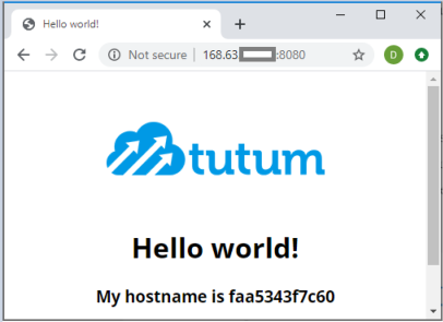
At this point, you can try to access this application using the public IP address which Azure allocated to the machine (or on your firewall) and running in a browser as follows:

http://<your_public_ip:8080/

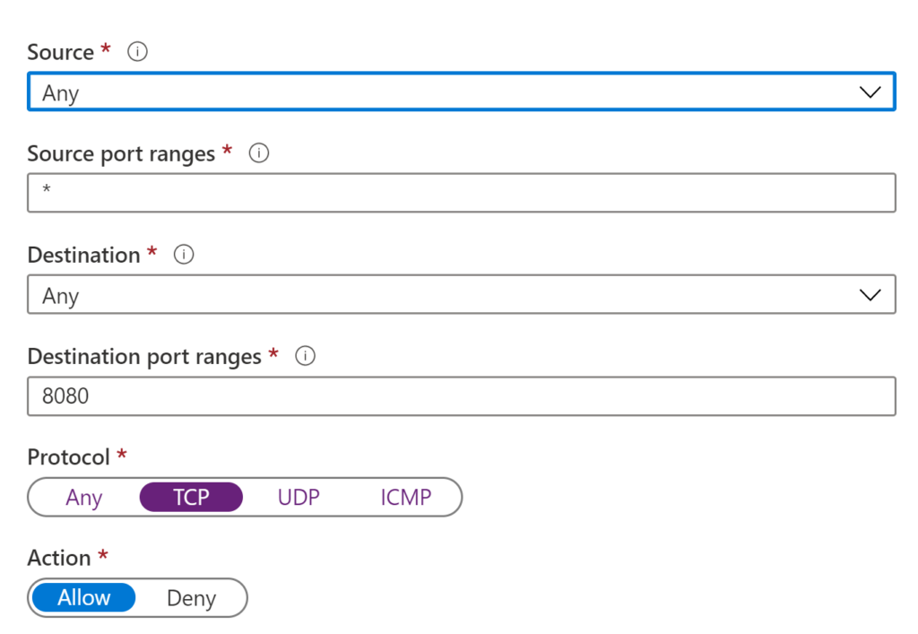
Note that if you’re getting a timeout form the browser, the 8080 port might to be allowed from the firewall. In my case since I’m using Azure, I went to Networking settings on the dashboard and enabled the inbound access as shown below.

Finally you should be able to reveal the demo web application project as follows.

Conclusion

In this article I went through some explanation on how to create your own dedicated hosting space with networking and host a simple application on it. I also introduced Docker a a powerful platform which can be used to simplify deploying new applications and services on your server.

In my next articles I will talk about building your own application and use Docker to containerise it and host it on your server. I will briefly explain how you can make a basic automatic deployment and continuous integration (CI-CD) pipeline so that you can continuously deploy updates of your application.

In a later article I will explain how an application can be made scalable and highly available so that when new updates are being deployed you have zero downtime.

Stay tuned for more!

References

1.Docker web demo container
https://hub.docker.com/r/tutum/hello-world/

2. Installing Docker on Ubuntu
https://docs.docker.com/engine/install/ubuntu/

Javascript

JS – The Last Stand Game

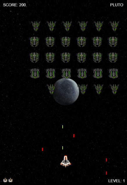
In recent years I decided I wanted to create a mini game using HTML 5 Canvas and pure JavaScript because I always wanted to understand how games work (the simple ones at least). Growing up in the 90’s I remember playing the infamous Space Invaders on the Nintendo and therefore I decided to create a spin off based on the same concept named The Last Stand.

The hero fighter space ship has to fight off waves of attacking aliens to regain control of the solar system. Each level gets harder as the intensity of the game increases and the levels are decorated and named after planets from Pluto to Mercury (yeah I know Pluto isn’t a planet) until the final battle takes place near the sun. In this post I will be going through the phases on how I went about developing this game and provide source code.

Live demo can be played [here].
*mobile not supported.

Please note you might need to zoom out on your browser to make it fit depending on screen size and resoltution. The game controls are simple: Left and Right arrow keys for movement and Space Bar for shooting.

Enjoy!

1. Canvas and Frames

The minimum you need to create an HTML 5 game is a canvas and two JavaScript methods: onload() where game objects like Sprites are loaded (more in this later) and loop() where things like rendering and object positions are updated or created into the canvas. Traditionally if you wanted to create a method which loops infinitely in JavaScript, you’d use the setInterval() function however modern browsers have something called requestAnimationFrame which can be used to provide a Frames per second loop which is more optimised for CPU and Battery use and also for smoother animation performance. The implementation of such method can be found [here].

The gameStart() method will load all the game objects and sprites and then the loop() method will be called. The loop() method itself calls requestAnimFrame(loop) which callbacks the method indefinitely creating a smooth FPS loop.

2. Game Sprites and Animations

In order to create object styles and animations, the most efficient way is to use Sprite images. In the base class I have created two methods: Sprite() and AnimationSprite(). The difference is that Sprite() will load the image with the coordinates given and remain a static non moving image whilst animated sprites will be loaded with multiple frames and played as a sequence kind of like a movie. To give an example, the explosion animation is loaded as an image sprite as follows and then played piece by piece to make it look like an organic fiery explosion.

Since I was having fun with JavaScript I decided to structure the code in a clean OOP and since these methods could apply to any other game, I placed this code in the base class [here]. The image assets which were used in this game were found online a few years back and my designer colleagues helped me with some touches, I don’t have references from where these were found but of course, many free resources can be found online or design your own.

3. Game Input Controls

The controls are pretty simple in this game: Enter to start, Left and Right to move and Space Bar to shoot. JavaScript event listeners were used to track the keyboard inputs, the code can be found [here]. At each loop iteration, the key input controls are read and actions are taken accordingly like changing the x and y position of an object on the canvas. For instance, the code responsible for moving the tank can be found [here].

4. Rendering

Objects inside the game are kept in distinct arrays and at each loop iteration, the canvas is cleared and rendered again. At each loop iteration, there are various methods being called which make checks (such as collision detection) and updates of animations or positions which make the game come to life. The update() method is responsible for calling all the update methods individually followed by the render() method which redraws all the sprite objects on canvas.

5. Collision Matrix

AABB Intersection (Axis-Aligned Bounding Box) is an algorithm used to determine whether objects on a 2D come to an intersection (or collision) at a given moment. Given the width, height, position x and position y of two objects, the AABBIntersect method calculates the collision matrix and returns true or false. This method is the real hero of the game since it’s able to intercept all hits being fired by the tank and the aliens ships at every loop cycle. When a collision is triggered. animations and sounds can be played accordingly to enhance the game experience.

6. Game-play design

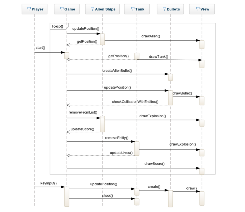
Below is a sequence diagram illustrating how the game works.

The aliens are programmed to move in a sequence to the side and down approaching the tank which is controller by the user. The alien ships produce a random shot attack (only if the alien ship is on front-line and not obstructed by other alien ships). The tank creates fire shots at the Space Bar press. The bullets follow a straight line trajectory and destroy any object which is encountered by calculating the collision matrix of each object at each loop cycle.

The score is updated at each successful hit and the level difficulty is increased when all aliens on canvas are cleared.

The full source code can be found [here].

7. Game Enhancements

For level design enhancement, THREE.JS framework can be used in order to create a background design with special effects containing planets in motion during the game-play such as I did here on the [live demo].

Also used Howler.js, a great framework for playing sound effects during the game using mp3 files.

Finally, I used geolocation tracking in the live demo (mostly because I wanted to experiment with this) and depending on the region you are from in the world, a different ship is generated.

Conclusion

In this post, it was demonstrated that with basic JavaScript and HTML 5 canvas a simple and pretty looking game can be created (if you happen to have good designer friends like myself).

So… how much score can you get? Go[here] to find out!.

References

1. Code Structuring tips for HTML 5 games
http://blog.sklambert.com/html5-game-tutorial-module-pattern/

2. Collision Matrix (AABB Intersection)
https://developer.mozilla.org/en-US/docs/Games/Techniques/2D_collision_detection

3. THREE.JS Framework (Planets)
https://github.com/jeromeetienne/threex.planets

4. Howler.JS JavaScript sound framework
https://github.com/goldfire/howler.js/

Tags Game, HTML, Javascript

AI Machine Learning

AI – Pattern Recognition

In my last [post ] I talked about Optical Character Recognition and how I managed to get a solution working using machine learning, particularly using the nearest neighbour algorithm. In this post I will briefly explain how the NN algorithm works and then introduce another two pattern recognition algorithms which I used to solve the OCR problem and compare their strengths and weaknesses.

Live demo can be accessed [here].

In a future article, I will implement the same algorithms using ML.NET and see if I get better results than my own implementations. So stay tuned!

1. Nearest Neighbour

The algorithm is based on a distance metric such as the Euclidean Distance which is used to find the closest similarity (nearest distance) among a set of vectors. Let’s assume in this case we have an array of integers and we want to compare this with other arrays of integers to determine which one is the most similar to our own array of integers. A loop would go through each of the arrays one by one and make a comparison using the following simple formula below to obtain the euclidean distance.

At each iteration, every integer from array 1 is represented as x and every integer from array 2 is represented as y. In C# code, the following formula would translate to something like [this]. By applying this formula to compare the array of integers against all the other arrays inside the data set, the array which produces the shortest distance as result is considered to be the most similar to our array and this is how it was possible to solve the OCR problem in my previous [post], hence by comparing the array of bits produced by the scribbling on a canvas against all the other OCR images inside the CSV files.

2. K-Nearest Neighbour (k-NN)

In combination with nearest neighbour, a very powerful solution which can be used to optimise the accuracy of the nearest neighbour is the k-NN algorithm; a non-parametric supervised learning method used for both classification and regression predictive problems.

The k-NN rather than classifying the nearest neighbour by shortest distance metric, it takes the closest K neighbours and forms a majority vote among them to determine which character occurs the most times (K being any number). So basically going back to the OCR problem, let’s imagine that “3” is the number we are trying to predict by using the Nearest Neighbour and we get Euclidean Distance of 0.2 on a character which is a “3” and 0.19 on a character that is an “8”. This can very much happen if the character is not written very clearly and thus it gets mistaken for a number with similar pattern attributes.

What the k-NN does basically, rather than choosing the result with shortest distance; it takes the top four or five (K) with shortest distance which are found. This way a vote can then be made and determine the likelihood from the majority. For the sake of our example, we could get the following for K=4:

{ 1.9 = “8”, 0.2 = “3”, 0.21 = “3”, 0.24 = “3” }

This means that although the result with shortest euclidean distance relative to our number is an 8, there are another 3 results which indicate it’s a 3 and therefore the majority vote concludes that it is in fact a 3. This improves slightly the predictive performance over the classical nearest neighbour. A C# implementation of the k-NN can be found [here].

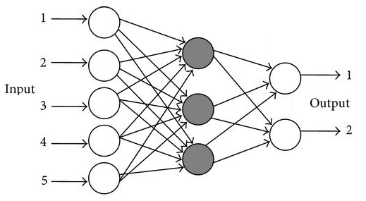
3. Multi-Layered Perceptron

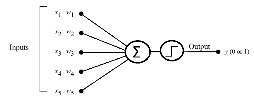
The Multi-Layered Perceptron originates from a single perceptron node which takes a set of input values as parameters and then produces a binary output (usually 0 or 1). At each input node, a randomly generated weight value (ex: -0.5 to +0.5) is set and multiplied to the input value. The totals are then summed together in a connecting node and finally the total is produced using the sigmoid function a.k.a the step function (or activation function).

Of course the perceptron approach works very well when dealing with linear separation for example when determining whether an object is a car or a truck (separating only 2 types), but in our case the OCR problem is more complex than that. For this reason, multiple perceptrons can be combined together to form a neural network which will be able to identify 10 different characters, hence produce 10 different output types.

This approach could work even if multiple middle layers (called hidden layers) could be connected in between each with their own weight value and values summed together from back to front (feed forward). However the a neural network is usually implemented with a back propagation function which goes backwards and corrects the values at each iteration during training phase in order to minimise the resulting error for that particular value and thus drastically improving the performance on the prediction results. Back propagation is quite complex to understand but many tutorials are available online which go in depth with the explanation.

For our OCR solution, a MLP algorithm classifier example in C# has been implemented and can be found [here]. The following configurations have been applied.

Input Layers (64): The OCR data is represented in a 64 bit binarised numeric value.
Output Layers (10): The possible classification of digits 0 – 9.
Hidden Layers (3): By trial and error it turns out 3 layers give the most accurate results.
Hidden Neurons (52): “The number of hidden neurons should be 2/3 of the input layer size, plus the size of the output layer”, Foram S.Panchal et al (2014).
Momentum (0.4): The coefficient value multiplied by the learning step which adds speed to the training of any multi-layer perceptron.
Learning Step (0.04): The constant used by algorithm for learning, 0.4 gave the best results while fine tuning although for smaller datasets 0.06 also worked very well.
Least Mean Square Error (0.01): The minimum error difference to get in training precision before stopping.
Epoch (500): The number of times to repeat the back-propagation during training to get the weights adjusted correctly. The higher the value the more precise the character recognition but the slower the performance. NB: Setting this value higher than 500 seems to make insignificant difference in the output accuracy for the data set which we are working with.
Function: Sigmoid function has been used as most practically used worldwide.

When passing the two-fold data through the perceptron, the training method might take a bit long to complete since it will need to iterate too many N times for each character given. For this reason filtering has been applied to limit the number of training data for each represented digit from 0 – 9 but is has been observed that the smaller the data set for training passed although it shortens the processing time, it reduces the percentage accuracy of the result.

Results Comparison

Below are the accuracy performance results based on a 2-fold test. But perhaps the accuracy can be tested manually on the live demo page [here]. Which one gets it right most of the time for your handwriting?

Algorithm	Performance	% Accuracy
KNN	2760 / 2810	98.22%
NN	2755 / 2810	98.04%
MLP	2727 / 2810	97.04%

Conclusion

The nearest neighbour and k-NN functions have shown by far the highest accuracy achievement in the smallest amount of running time however such algorithms, being non-parametric kind; lack the ability to learn and therefore their processing requires a training dataset to be available at all time. On the other hand, the multilayer perceptron is able to learn and produce a neural network with adjusted weights over a span of time which then uses to classify characters without the need to the original training set.

Although such method takes a very long time to run compared to the other methods, the weight adjustment values can be saved in a file after the training has been completed and then use only the saved adjusted weights from the file to run the OCR classification almost instantly. Theoretically, the MLP method has also the potential that more accuracy can be achieved when fed a larger training dataset and finer tuning of the other parameters such as epoch and learning step.

References

1. Multi-layer Perceptron Tutorial
http://blog.refu.co/?p=931

2. Multi-Layer Neural Networks with Sigmoid Function
https://towardsdatascience.com/multi-layer-neural-networks-with-sigmoid-function-deep-learning-for-rookies-2-bf464f09eb7f/

3. Review on Methods of Selecting Number of Hidden Nodes in Artificial Neural Network
http://www.ijcsmc.com/docs/papers/November2014/V3I11201499a19.pdf

Tags AI, MachineLearning, PatternRecognition

AI Machine Learning

Creating a hand written number recognition program using machine learning

Post author By dgrixti
Post date 3 May 2020
1 Comment on Creating a hand written number recognition program using machine learning

Back when I was studying AI and Machine Learning, I was given an assignment where I had to create an Optical Character Recognition (OCR) program using the MNIST (http://yann.lecun.com/exdb/mnist/) data set. The requirement was to create a couple of Machine Learning algorithms such as Nearest Neighbour and Multi-Layred Perceptron (more on these later) and then run a two-fold test through these algorithms to train a model to for classifying hand-written digits. The first half of the data set would be used to train the model and the second half to test the outcome prediction for the given characters ultimately calculating the percentage of accuracy in the results.
I wanted to take this a step further and create a GUI where a user could hand-write a digit and the program would try guessing the input by learning from the data set.

Check out the live demo [here].

Step 1: Examining Data

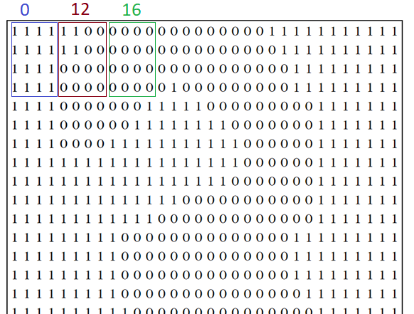
The training data which we will be working with is in CSV format and each row contains a set of 65 integer values, the first 64 being the data bits (vectors) representing the character and the last being the actual identifier (a character between 0 – 9). The data set can be found [here]. The scanned numbers have been converted from image bitmaps to 32×32 pixel format, kind of like a grid of ON and OFF values which depict the character black on white. These ON and OFF values are represented as 0s and 1s and then these bits are divided into 4×4 non-overlapping blocks.

The number of ON pixels is counted in each of these blocks to give a value between 1 and 16. This part is explained in more detail later but for now, the idea is to understand the format of the train data in order to create the same format when inserting the hand-drawn values into the program.

The SUM of each 4×4 block give the 64 bit integer sequence which will be representation of the character (0-9).

Step 2: Canvas to Pixels

The goal is to create a canvas onto which a user could write a digit using mouse or touch-pad and convert the bitmap into the same 64 bit sequence in order to run through a machine learning algorithm to predict the most likelihood of the character compared to the rest of the training data set. If we had to provide a 32×32 pixel canvas, it would be a bit too tiny to allow any scribbling as input and therefore we will create a 100×100 pixel canvas and then resize it later using a preview canvas. The code for creating user scribbling on an HTML canvas and then resizing can be found on Github [here].

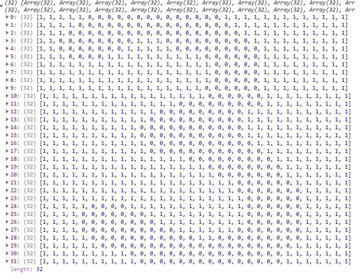
When processing the canvas data, it’s vital to understand how pixels work. Each pixel is repented by 4 values: Red, Blue, Green and Alpha. I won’t get too much into detail on this since it can be looked up easily but basically for our sake, the important thing to know is that when dealing with raw canvas data, each sequence of 4 characters = 1 pixel. In this case, 32×32 pixels = 1024 bits * 4 = 4096; below is the console log of canvas.data illustrated.

The convertToGrascaleMatrix() method, loops through all these pixels and organises them into a 32×32 pixel grid array. In each iteration, the Alpha value (4th bit) is checked whether it’s a 0 (OFF) or any value between 1-255 (ON) and 1 or 0 is inserted in the array accordingly. Below is the console log of the end result, the binary output resembles the drawn image.

The next step is to send the pixels array into the count4X4MatrixSections() to create the 4×4 blocks and count the ON /OFF values inside and produce the 64 bit integer sequence to send into the machine learning algorithm.

Example in this case: 3,15,14,15,15,3,0,0,3,7,1,2,11,12,0,0,0,0,0,2,12,12,0,0,0,0,5,16,16,4,0,0,0,0,2,9,15,13,1,0,0,0,0,0,2,15,9,0,0,15,12,2,0,13,12,0,0,5,13,16,14,16,7,0,

Step 3: Machine Learning

The nearest neighbour algorithm is a good starting place for attempting to resolve the OCR problem as it will use a distance function to calculate the distance between the sums of the vectors of a given OCR character (in our case the 64 bit integers) against those in the training data set and classify the number according to its closes neighbour’s identifier. I won’t get too much into detail about the algorithm itself since I will be doing another [article] about machine learning algorithms soon, plus Google is your friend if you wish to look up the nearest neighbour algorithm and euclidean distance.

For this project, I chose to implement this algorithm and use Euclidian Distance as the distance function to predict the inserted characters. The code is in C# and can be found [here] with inline comments explaining the behaviour at each step.

Step 4: Refining Results

When I finished the first version of this project, I was getting pretty good result predictions from the algorithm but when I asked some friends to try it, the results weren’t so accurate anymore. I realised after some analysis that when I was writing the characters on the canvas I was drawing big numbers to occupy all the space in the box whilst other people weren’t.

I concluded that since the OCR training data-set is based on bitmaps of numbers which are centered and without much white bordering and white space in general that it would be a good idea to introduce a certalise and crop function in order to give the algorithm more refined data to work with. The centraliseAndCropCanvas() method is based on a few concepts which I found by research and adapted to my project, I will leave references for these below. Basically finding the bounding rectangle in the image eliminates the outer white spaces and then finding the center of mass of the character helps repositioning the character at the middle of the canvas after the cropping.

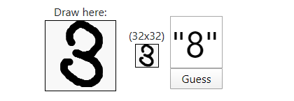
The code for these functions can be found in this JavaScript file [here]. This has drastically improved the performance of the algorithm. The preview box illustrates the final version of the drawn up character after undergoing all transformation and before being sent to the algorithm.

Conclusion

Of course, it can never reach a 100% accuracy but if you think about it, even a human being can have difficulty recognising a handwritten digit every now and then let alone a machine!

You want to try yourself? Check out the demo [here].

Full source code can be found on [Github].

What next?

I will make another [post] where I will compare other algorithms such as the kNN and the Multi-Layered Perceptron and discuss the advantages and disadvantages and try to apply the GUI created in this project on them.

Also I will be trying the ML.NET libraries for machine learning and apply the GUI to check if I get better results than my own.